Example of video data labeling using k-means clustering with a color histogram – Exploring Video Data

Let us see example code for performing k-means clustering on video data using the open source scikit-learn Python package and the Kinetics human action dataset. This dataset is available at GitHub path specified in the Technical requirements section.

This code performs K-means clustering on video data using color histogram features. The steps include loading video frames from a directory, extracting color histogram features, standardizing the features, and clustering them into two groups using K-means.

Let’s see the implementation of the steps with the corresponding code snippet:

1. Load videos and preprocess frames: Load video frames from a specified directory. Resize frames to (64, 64), normalize pixel values, and create a structured video dataset:

input_video_dir = “/PacktPublishing/DataLabeling/ch08/kmeans/kmeans_input”
input_video, _ = load_videos_from_directory(input_video_dir)

2. Extract color histogram features: Convert each frame to the HSV color space. Calculate histograms for each channel (hue, saturation, value). Concatenate the histograms into a single feature vector:

hist_features = extract_histogram_features( \
input_video.reshape(-1, 64, 64, 3))

3. Standardize features: Standardize the extracted histogram features using StandardScaler to have zero mean and unit variance:

scaler = StandardScaler()
scaled_features = scaler.fit_transform(hist_features)

4. Apply K-means clustering: Use K-means clustering with two clusters on the standardized features. Print the predicted labels assigned to each video frame:

kmeans = KMeans(n_clusters=2, random_state=42)
predicted_labels = kmeans.fit_predict(scaled_features)
print(“Predicted Labels:”, predicted_labels)

This code performs video frame clustering based on color histogram features, similar to the previous version. The clustering is done for the specified input video directory, and the predicted cluster labels are printed at the end.

We get the following output:

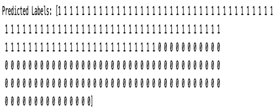
Figure 8.5 – Output of the k-means predicted labeling

Now write these predicted label frames to the corresponding output cluster directory.

The following code flattens a video data array to iterate through individual frames. It then creates two output directories for clusters (Cluster_0 and Cluster_1). Each frame is saved in the corresponding cluster folder based on the predicted label obtained from k-means clustering. The frames are written as PNG images in the specified output directories:
# Flatten the video_data array to iterate through frames
flattened_video_data = input_video.reshape(-1, \
    input_video.shape[-3], input_video.shape[-2], \
    input_video.shape[-1])
# Create two separate output directories for clusters
output_directory_0 = “/<your_path>/kmeans_output/Cluster_0”
output_directory_1 = “/<your_path>/kmeans_output/Cluster_1”
os.makedirs(output_directory_0, exist_ok=True)
os.makedirs(output_directory_1, exist_ok=True)
# Iterate through each frame, save frames in the corresponding cluster folder
for idx, (frame, predicted_label) in enumerate( \
    zip(flattened_video_data, predicted_labels)):
    cluster_folder = output_directory_0 if predicted_label == 0 else output_directory_1
    frame_filename = f”video_frame_{idx}.png”
    frame_path = os.path.join(cluster_folder, frame_filename)
    cv2.imwrite(frame_path, (frame * 255).astype(np.uint8))

Now let’s plot to visualize the frames in each cluster. The following code visualizes a few frames from each cluster created by K-means clustering. It iterates through the Cluster_0 and Cluster_1 folders, selects a specified number of frames from each cluster, and displays them using Matplotlib. The resulting images show frames from each cluster with corresponding cluster labels:
# Visualize a few frames from each cluster
num_frames_to_visualize = 2
for cluster_label in range(2):
    cluster_folder = os.path.join(“./kmeans/kmeans_output”, \
        f”Cluster_{cluster_label}”)
    frame_files = os.listdir(cluster_folder)[:num_frames_to_visualize]
    for frame_file in frame_files:
        frame_path = os.path.join(cluster_folder, frame_file)
        frame = cv2.imread(frame_path)
        frame = cv2.cvtColor(frame, cv2.COLOR_BGR2RGB)
        plt.imshow(frame)
        plt.title(f”Cluster {cluster_label}”)
        plt.axis(“off”)
        plt.show()

We get the output for cluster 0 as follows:

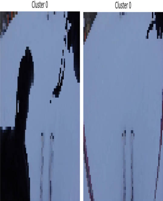
Figure 8.6 – Snow skating (Cluster 0)

And we get the following output for cluster 1:

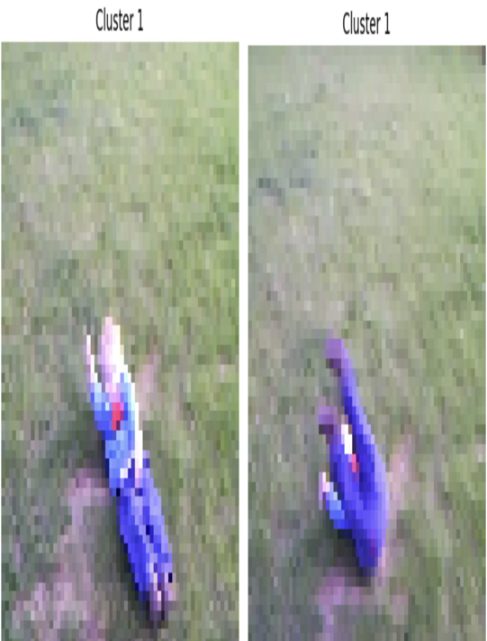
Figure 8.7 – Child play (Cluster 1)

In this section, we have seen how to label the video data using k-means clustering and clustered videos into two classes. One cluster (Label: Cluster 0) contains frames of a skating video, and the second cluster (Label: Cluster 1) contains the child play video.

Now let’s see some advanced concepts in video data analysis used in real-world projects.