Exploratory data analysis of sample text data set – Labeling Text Data

Here’s an example Python code for performing EDA on a text dataset. We will be using the Gutenberg corpus (https://pypi.org/project/Gutenberg/), which is a publicly available collection of over 60,000 electronic books.

The NLTK corpus is a collection of publicly available datasets for NLP research and development. The Gutenberg corpus (https://www.nltk.org/book/ch02.html), which is one of the datasets included in NLTK, specifically contains a selection of public domain texts from Project Gutenberg. Project Gutenberg is a digital library that offers free access to books and other texts that are no longer protected by copyright.

Therefore, the Gutenberg corpus within the NLTK is based on public domain texts, making it a publicly available dataset. It can be used for various NLP tasks, such as text classification, language modeling, and information retrieval, without any commercial restrictions or licensing requirements:
import nltk
from nltk.corpus import gutenberg
import string
import pandas as pd
import numpy as np
import matplotlib.pyplot as plt
import seaborn as sns

Let’s download the Gutenberg corpus using the NLTK library:
# Download the Gutenberg corpus
nltk.download(‘gutenberg’)

Let’s load the text data into a Pandas DataFrame by iterating the fields from Gutenberg and appending documents to the list data. Then we’ll convert the list data to dataframe, df, with a single column, text, to store the document:
# Load the data
data = []
for file_id in gutenberg.fileids():
    document = ‘ ‘.join(gutenberg.words(file_id))
    data.append(document)
df = pd.DataFrame(data, columns=[‘text’])
# View the first few rows of the data
print(df.head())

Let’s check the dataframe’s size by calling the shape function:

Here’s the output:
# Check the size of the dataset
print(“Dataset size:”, df.shape)

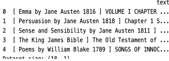
Figure 7.1 – The first few rows of data

Let’s check the length of each document by calling the apply function:
# Check the length of each document
df[‘text_length’] = df[‘text’].apply(len)
 Let us plot the histogram plot of the ‘text_length’ column using seaborn library sns.
# Visualize the distribution of document lengths
plt.figure(figsize=(8, 6))
sns.distplot(df[‘text_length’], bins=50, kde=False, color=’blue’)
plt.title(‘Distribution of Text Lengths’)
plt.xlabel(‘Text Length’)
plt.ylabel(‘Count’)
plt.show()

Here’s the output:

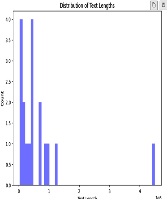
Figure 7.2 – Distribution of document length

In text analysis, removing stopwords and punctuation is one of the most common tasks because stopwords do not tell us anything about the text:
# Remove punctuation and stop words
def remove_punctuation(text):
    return text.translate(str.maketrans(”, ”, string.punctuation))

We will use the stopwords list from the NLTK corpus:
def remove_stopwords(text):
    stopwords_list = nltk.corpus.stopwords.words(‘english’)
    return ” “.join([word for word in text.split() if \
        word.lower() not in stopwords_list])
df[‘text_clean’] = df[‘text’].apply(remove_punctuation)
df[‘text_clean’] = df[‘text_clean’].apply(remove_stopwords)

Now let’s count the frequency of words in the clean text using the value_counts function:
# Count the frequency of each word
word_freq = pd.Series(np.concatenate([x.split() for x in \
    df[‘text_clean’]])).value_counts()

Finally, plot a bar chart to visualize the most frequent words:
# Visualize the most frequent words
plt.figure(figsize=(12, 8))
word_freq[:20].plot(kind=’bar’, color=’blue’)
plt.title(‘Most Frequent Words’)
plt.xlabel(‘Word’)
plt.ylabel(‘Frequency’)
plt.show()

Here’s the output:

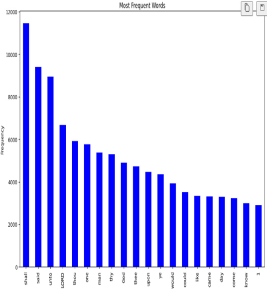
Figure 7.3 – Most frequent words

In this code, we first downloaded the Gutenberg corpus using the NLTK library. We then loaded the text data into a Pandas DataFrame and performed some initial checks on the size and structure of the dataset.

Next, we calculated the length of each document and visualized the distribution of document lengths using a histogram. We then removed punctuation and stop words from the text data and calculated the frequency of each word. We visualized the most frequent words using a bar chart.

Note that this code is just a basic example of EDA on text data, and you may need to modify it to suit your specific dataset and research question. Now we have clean text data.

Let’s see how to use Generative AI to label text data in the following section.